This is the first part of a series building a privacy-first RAG system with open-source LLMs from HuggingFace (using Ollama), LangChain and Chroma.
At the end of this blog series, we will have a fully functioning, production-ready RAG system for your company or organization.
In this tutorial, everything will run locally as our main goal is to keep the data private within your organization. On the last section, we will suggest some improvements in case you are willing to sacrifice privacy for performance and scalability.
Series Index
- Prerequisites
- Populate the Vector Database
- Vector Retriever
- RAG Implementation
- Chat UI
- Evaluation
- Performance improvements
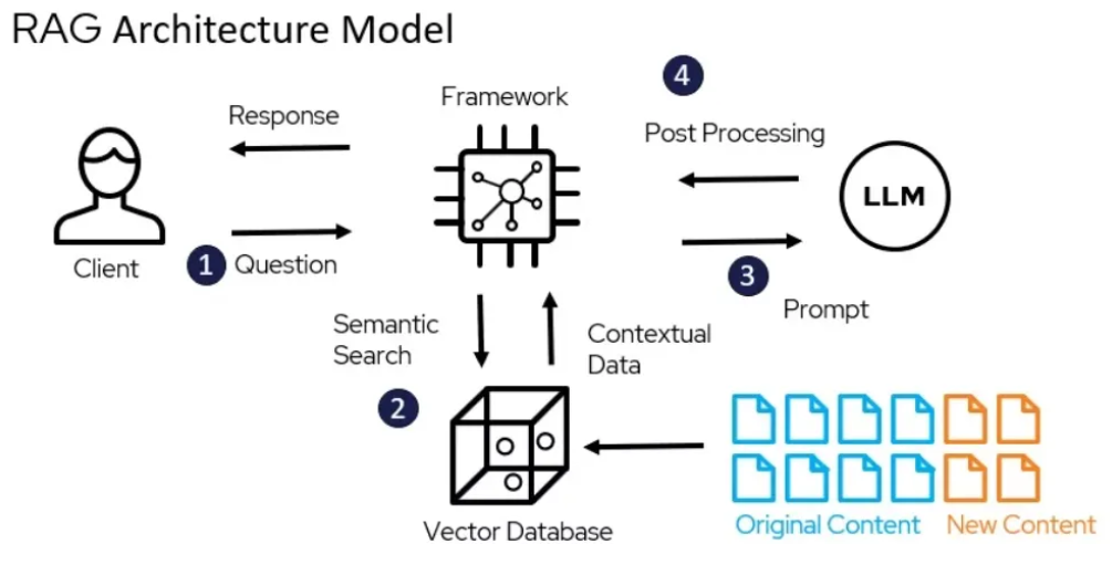
How a RAG System Works (High Level)

1. Prerequisites
We assume the knowledge base is already organized in folders and stored in Markdown (.md) files.
If you’re just getting started or don’t yet have structured data, check the post on how to generate synthetic datasets (TODO) or get one from HuggingFace .
2. Populate the Vector Database
What Is a Vector?
A vector is a multi-dimensional numerical representation of text. It encodes semantic meaning into coordinates inside a high-dimensional space. We’ll visualize these embeddings later.
The pipeline is simple:
- Split documents into chunks.
- Generate embeddings for each chunk.
- Store them in a vector database.
2.1 Split the Knowledge Base into Chunks
Given an array of documents called documents:
from langchain_text_splitters import RecursiveCharacterTextSplitter

text_splitter = RecursiveCharacterTextSplitter(chunk_size=3200, chunk_overlap=480)
chunks = text_splitter.split_documents(documents)
Two parameters matter:
chunk_size: number of characters per chunk.chunk_overlap: overlap between consecutive chunks.
A common standard is 800 tokens, which equals roughly 3200 characters (1 token ≈ 4 characters).
We will optimise further on the evaluation section to find the sweet-spot between:
- Chunks too short → context fragmentation
- Chunks too long → retrieval noise
Recommended overlap:
- Light overlap (facts, code, structured text): 10–15%
- Heavy overlap (legal, narrative, procedural): 20–30%
For general company documentation, 15% works well:
chunk_size = 3200
chunk_overlap = int(chunk_size * 0.15)  # 480
2.2 Generate Embeddings
Now we create embeddings using an encoder model. These models differ from autoregressive LLMs—they do not generate text but instead convert text into dense vector representations.
Example using HuggingFace:
from langchain_community.embeddings import HuggingFaceEmbeddings
# from langchain_openai import OpenAIEmbeddings

embeddings = HuggingFaceEmbeddings(model_name="sentence-transformers/all-MiniLM-L6-v2")
# embeddings = OpenAIEmbeddings(model="text-embedding-3-large")
For commercial applications, OpenAI’s text-embedding-3-small and
text-embedding-3-large give higher accuracy at a slightly higher cost.
2.3 Store the Embeddings in Chroma
from langchain_community.vectorstores import Chroma
import os

DB_NAME = "company_rag_chroma"

# Reset collection if it already exists
if os.path.exists(DB_NAME):
    Chroma(persist_directory=DB_NAME, embedding_function=embeddings).delete_collection()

vectorstore = Chroma.from_documents(
    documents=chunks,
    embedding=embeddings,
    persist_directory=DB_NAME,
)
At this point, the vector database is populated.
To inspect it:
collection = vectorstore._collection
count = collection.count()

sample_embedding = collection.get(limit=1, include=["embeddings"])["embeddings"][0]
dimensions = len(sample_embedding)

print(f"There are {count:,} vectors with {dimensions:,} dimensions in the vector store")
Example output:
There are 413 vectors with 384 dimensions in the vector storeThis means we have 413 chunks represented in a 384-dimensional space.
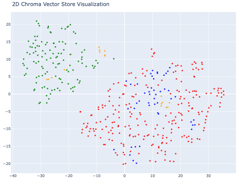
2.4 Visualizing Embeddings in 2D
Although impossible to understand high-dimensional space directly, we can reduce it using t-SNE.
import numpy as np
from sklearn.manifold import TSNE
import plotly.graph_objects as go

result = collection.get(include=["embeddings", "documents", "metadatas"])
vectors = np.array(result["embeddings"])
documents = result["documents"]
metadatas = result["metadatas"]

# Example: color by document type
DOC_TYPES = ["products", "employees", "contracts", "company"]
COLORS = ["blue", "green", "red", "orange"]

doc_types = [metadata["doc_type"] for metadata in metadatas]
colors = [COLORS[DOC_TYPES.index(t)] for t in doc_types]
Reduce to 2D:
tsne = TSNE(n_components=2, random_state=42)
reduced_vectors = tsne.fit_transform(vectors)
Plot:
fig = go.Figure(data=[go.Scatter(
    x=reduced_vectors[:, 0],
    y=reduced_vectors[:, 1],
    mode="markers",
    marker=dict(size=5, color=colors, opacity=0.8),
    text=[f"Type: {t}<br>Text: {d[:100]}..." for t, d in zip(doc_types, documents)],
    hoverinfo="text",
)])

fig.update_layout(title="2D Chroma Vector Store Visualization")
fig.show()
We observe a strong relation between products and contracts. An a softer one between company and emproyees/products.
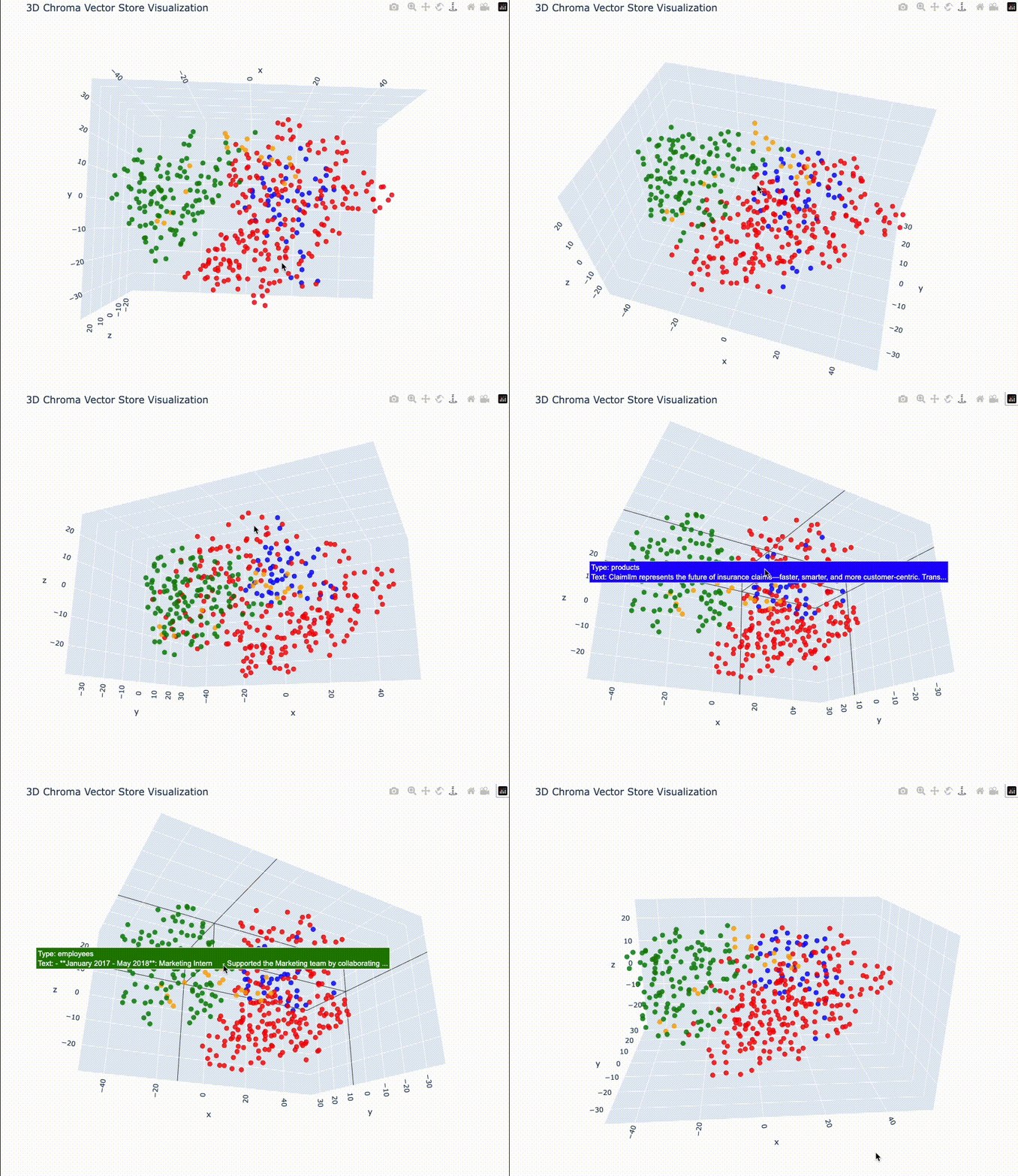
2.5 Visualizing Embeddings in 3D
tsne = TSNE(n_components=3, random_state=42)
reduced_vectors = tsne.fit_transform(vectors)

fig = go.Figure(data=[go.Scatter3d(
    x=reduced_vectors[:, 0],
    y=reduced_vectors[:, 1],
    z=reduced_vectors[:, 2],
    mode="markers",
    marker=dict(size=5, color=colors, opacity=0.8),
    text=[f"Type: {t}<br>Text: {d[:100]}..." for t, d in zip(doc_types, documents)],
    hoverinfo="text",
)])

fig.update_layout(
    title="3D Chroma Vector Store Visualization",
    scene=dict(xaxis_title="x", yaxis_title="y", zaxis_title="z"),
    width=900,
    height=700,
    margin=dict(r=10, b=10, l=10, t=40)
)

fig.show()
Good job! Only with this, we got roughly 25% of our private RAG system.
We are ready now to move to the next part: Part 3: Create the vector retriever
More LLM Engineering articles
- LLM Engineering | Token optimization – caching, thin system prompts, and cost-optimized production usage.
- LLM Engineering | Running local LLMs and APIs – Ollama, OpenAI, Anthropic, OpenRouter, LangChain, and LiteLLM.